Understanding Gradient Descent in Depth

Oct 16, 2024

What is Gradient Descent?

Gradient Descent is an optimization algorithm used to minimize the loss function in machine learning and deep learning models. It iteratively adjusts the model's parameters to find the minimum of a cost function by moving in the direction opposite to the gradient of the cost function (hence the name "descent").

The key idea is that, given a cost function J(θ), where θ represents the model's parameters, the algorithm updates θ in the opposite direction of the gradient of J(θ) with respect to θ to minimize the error.

Why Do We Use Gradient Descent?

Minimizing Loss: In machine learning, we aim to minimize a loss (or cost) function that represents how well the model is performing. Gradient Descent helps in finding the optimal set of parameters that lead to the lowest possible error.
Training Neural Networks: Gradient Descent is widely used to optimize weights in deep learning models (neural networks) by minimizing the error between predicted and actual values.
Efficiency in High Dimensions: For high-dimensional datasets, gradient descent is computationally efficient compared to other optimization algorithms.

Use Cases of Gradient Descent

Linear Regression: Gradient Descent helps to find the line of best fit by minimizing the Mean Squared Error (MSE) between predicted and actual values.
Logistic Regression: Used for binary classification problems to minimize the logistic loss function.
Neural Networks: It is the backbone of training deep learning models by optimizing weights across layers of the network.
Support Vector Machines (SVM): Used for optimizing the cost function in SVMs for classification tasks.
Clustering Algorithms (K-Means): Gradient descent helps in minimizing intra-cluster distances to optimize the cluster centroids.

What is a Loss Function?

A loss function measures the error or difference between the predicted output of a machine learning model and the actual output. It quantifies how "wrong" the model's predictions are for a single data point. The goal of training the model is to minimize this loss by adjusting the model's parameters (e.g., weights and biases).

Example: In a regression problem, a common loss function is the Mean Squared Error (MSE), which measures the squared difference between the predicted and actual values.
In classification problems, the Cross-Entropy Loss (also called log loss) is commonly used, which measures the difference between the predicted probability distribution and the actual distribution.

What is a Cost Function?

A cost function represents the average or aggregate loss over the entire dataset. It is the function that Gradient Descent tries to minimize by adjusting the model parameters. In other words, the cost function is the overall measure of error for the entire dataset, while the loss function computes the error for a single example.

Cost function is often referred to as the "objective function" in optimization problems, and minimizing the cost function is the ultimate goal during model training.
The cost function is typically the sum or average of the individual losses calculated for each data point.

Why is the Cost Function Important?

The cost function is crucial because it gives us a sense of how well or poorly the model is performing across all the training data. The goal of optimization techniques like Gradient Descent is to minimize the cost function by adjusting the model's parameters, thereby improving the model's accuracy.

Summary of Difference Between Loss and Cost Function:

Loss function measures the error for a single training example (or data point).
Cost function is the average or sum of all the loss values across the entire dataset.

Gradient Descent: Predicting House Prices

Let's consider a real-world scenario where we want to predict house prices based on some features like the size of the house (in square feet). The problem is a linear regression problem, and we will use Gradient Descent to optimize the parameters (slope and intercept) of the linear regression model to predict house prices accurately.

Problem Statement

Given a dataset with house sizes and corresponding prices, we want to predict the price of a house based on its size using a linear relationship between house size and price. To achieve this, we'll optimize the parameters (slope and intercept) of a linear regression model using Gradient Descent.

Price = m × Size + c

Where:

m is the slope (weight of size).
c is the intercept (bias).

Step 1: Generate Synthetic Data for House Sizes and Prices

np.random.seed(42)
house_size = np.random.rand(100) * 2000  # House sizes between 0 and 2000 sq ft
house_price = 100 + house_size * 250 + np.random.randn(100) * 50000  # Adding some noise

Here we generate synthetic data using:

np.random.rand(100) * 2000: Creates 100 random house sizes between 0 and 2000 sq ft.
house_price: Uses a linear equation price = 100 + size × 250 with some random noise added to make it more realistic. The noise simulates variability in house prices that cannot be explained solely by size.

Step 2: Initialize Parameters

m = 0  # Initial slope (weight)
c = 0  # Initial intercept (bias)
learning_rate = 0.0000001  # Learning rate
iterations = 1000  # Number of iterations

We initialize the slope (m) and intercept (c) to zero. These will be adjusted during the gradient descent process.
Learning rate is a small positive number that controls the size of the steps we take towards minimizing the cost function. A small learning rate ensures convergence, while a large one might overshoot the minimum.
Iterations defines how many times we’ll update the model parameters (m and c).

Step 3: Define the Cost Function

def compute_cost(size, price, m, c):
    n = len(size)
    predicted_price = m * size + c
    cost = (1/n) * np.sum((predicted_price - price) ** 2)
    return cost

This function calculates the Mean Squared Error (MSE), which represents the difference between the predicted prices and actual prices:

n is the number of data points.
predicted_price = m × size + c is the predicted price using the current slope and intercept.
We calculate the sum of squared differences between the predicted and actual prices, divide by the number of points n, and return the cost.

Step 4: Gradient Descent Algorithm

def gradient_descent(size, price, m, c, learning_rate, iterations):
    n = len(size)
    cost_history = []
    
    for i in range(iterations):
        predicted_price = m * size + c
        dm = -(2/n) * np.sum(size * (price - predicted_price))  
        # Gradient w.r.t. m
        dc = -(2/n) * np.sum(price - predicted_price)  # Gradient w.r.t. c
        
        # Update m and c using gradients
        m = m - learning_rate * dm
        c = c - learning_rate * dc
        
        # Calculate the cost and store it for plotting
        cost = compute_cost(size, price, m, c)
        cost_history.append(cost)
        
        # Print the cost every 100 iterations
        if i % 100 == 0:
            print(f"Iteration {i+1}: Cost = {cost}, m = {m}, c = {c}")
    
    return m, c, cost_history

How Gradient Descent Works:

For each iteration: We calculate the predicted price using the current values of m (slope) and c (intercept).
We compute the gradients:
- ∂J/∂m (gradient w.r.t slope): Measures how much the cost would change if we tweak the slope.
- ∂J/∂c (gradient w.r.t intercept): Measures how much the cost would change if we tweak the intercept.
Update m and c: We subtract the product of the learning rate and gradient from the current values of m and c, moving them toward values that minimize the cost function.
We store the cost after each iteration for visualization.

Step 5: Perform Gradient Descent to Find Optimal `m` and `c`

m, c, cost_history = gradient_descent(house_size, house_price, m, c, learning_rate, iterations)

Here we call the gradient_descent() function to perform the optimization and get the optimized values for m (slope) and c (intercept), along with the history of the cost function over the iterations.

Step 6: Display Final Values of `m` and `c`

print(f"Optimized Slope (m): {m}")
print(f"Optimized Intercept (c): {c}")

This prints the final optimized values for the slope and intercept, which represent the line of best fit for predicting house prices based on size.

Step 7: Visualizing the Cost Function Over Iterations

plt.plot(range(iterations), cost_history)
plt.xlabel('Iterations')
plt.ylabel('Cost (Mean Squared Error)')
plt.title('Cost Reduction Over Time')
plt.show()

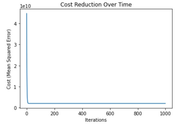
This code plots the reduction in the cost function (Mean Squared Error) over time. As the number of iterations increases, the cost decreases, indicating that the model is getting better at predicting house prices.

Step 8: Plotting House Sizes vs Actual and Predicted Prices

plt.scatter(house_size, house_price, color='red', label='Actual Prices')
plt.plot(house_size, m * house_size + c, color='blue', label='Predicted Prices')
plt.xlabel('House Size (sq ft)')
plt.ylabel('House Price')
plt.title('House Size vs Price')
plt.legend()
plt.show()

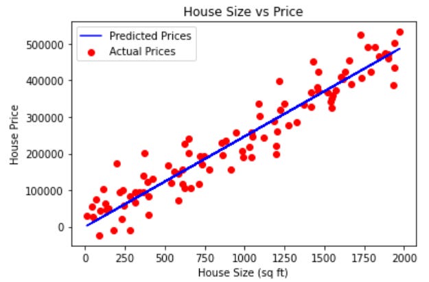
Finally, we visualize the actual house prices (red scatter plot) and the predicted prices (blue line) using the optimized values of m and c. The blue line is the best-fit line that Gradient Descent has calculated.

Iteration 1: Cost = 44690073540.138016, m = 60.93996409378216, c = 0.04702727073614737
Iteration 101: Cost = 2049903015.6354632, m = 246.772360513748, c = 0.25017263385034777
Iteration 201: Cost = 2049902635.9646027, m = 246.77231358680442, c = 0.3117900544070918
Iteration 301: Cost = 2049902256.298052, m = 246.77226666003776, c = 0.37340712518383
Iteration 401: Cost = 2049901876.6358125, m = 246.77221973353753, c = 0.4350238461826165
Iteration 501: Cost = 2049901496.9778824, m = 246.7721728073037, c = 0.4966402174054368
Iteration 601: Cost = 2049901117.3242626, m = 246.7721258813362, c = 0.5582562388542757
Iteration 701: Cost = 2049900737.6749542, m = 246.7720789556351, c = 0.6198719105311198
Iteration 801: Cost = 2049900358.0299554, m = 246.7720320302004, c = 0.6814872324379538
Iteration 901: Cost = 2049899978.389267, m = 246.7719851050321, c = 0.7431022045767638
Optimized Slope (m): 246.77193864937783
Optimized Intercept (c): 0.8041006824571423

Complete Code

import numpy as np
import matplotlib.pyplot as plt

# Step 1: Generate synthetic data for house sizes and prices
np.random.seed(42)
house_size = np.random.rand(100) * 2000  # House sizes between 0 and 2000 sq ft
house_price = 100 + house_size * 250 + np.random.randn(100) * 50000  # Adding some noise

# Step 2: Initialize parameters (slope 'm' and intercept 'c')
m = 0  # Initial slope (weight)
c = 0  # Initial intercept (bias)
learning_rate = 0.0000001  # Learning rate
iterations = 1000  # Number of iterations

# Step 3: Define the cost function (Mean Squared Error)
def compute_cost(size, price, m, c):
    n = len(size)
    predicted_price = m * size + c
    cost = (1/n) * np.sum((predicted_price - price) ** 2)
    return cost

# Step 4: Gradient Descent algorithm
def gradient_descent(size, price, m, c, learning_rate, iterations):
    n = len(size)
    cost_history = []
    
    for i in range(iterations):
        predicted_price = m * size + c
        dm = -(2/n) * np.sum(size * (price - predicted_price))  # Gradient w.r.t. m
        dc = -(2/n) * np.sum(price - predicted_price)  # Gradient w.r.t. c
        
        # Update m and c using gradients
        m = m - learning_rate * dm
        c = c - learning_rate * dc
        
        # Calculate the cost and store it for plotting
        cost = compute_cost(size, price, m, c)
        cost_history.append(cost)
        
        # Print the cost every 100 iterations
        if i % 100 == 0:
            print(f"Iteration {i+1}: Cost = {cost}, m = {m}, c = {c}")
    
    return m, c, cost_history

# Step 5: Perform Gradient Descent to find optimal m and c
m, c, cost_history = gradient_descent(house_size, house_price, m, c, learning_rate, iterations)

# Step 6: Display final values of m and c
print(f"Optimized Slope (m): {m}")
print(f"Optimized Intercept (c): {c}")

# Step 7: Visualizing the cost function over iterations
plt.plot(range(iterations), cost_history)
plt.xlabel('Iterations')
plt.ylabel('Cost (Mean Squared Error)')
plt.title('Cost Reduction Over Time')
plt.show()

# Step 8: Plotting the house sizes vs actual and predicted prices
plt.scatter(house_size, house_price, color='red', label='Actual Prices')
plt.plot(house_size, m * house_size + c, color='blue', label='Predicted Prices')
plt.xlabel('House Size (sq ft)')
plt.ylabel('House Price')
plt.title('House Size vs Price')
plt.legend()
plt.show()

Output Explanation

Cost Reduction Plot:
- This plot shows how the cost decreases over time as the algorithm optimizes the model. Initially, the cost is high, but as the model adjusts the parameters m and c, the cost reduces gradually and stabilizes, indicating convergence.
Final Values of m and c:
- After 1000 iterations, the final optimized values of m (slope) and c (intercept) are printed. These values define the line of best fit.
House Size vs. Price Plot:
- The red points represent the actual house prices, and the blue line represents the predicted prices using the optimized linear regression model. Ideally, the blue line should pass through or close to most of the red points, showing that the model is making reasonable predictions.

Few FAQ’s

What is a Hyperparameter?

A hyperparameter is a configuration or setting used to control the learning process of a machine learning algorithm. Hyperparameters are not learned by the model itself but are set before training begins. They influence how the model learns and performs during training, and their values are chosen by the user.

Common hyperparameters include:

Learning rate: Controls how fast or slow the model updates its parameters. In simpler terms, it dictates the size of the steps taken towards minimizing the cost function.
Number of iterations/epochs: Determines how many times the model will process the entire training data.
Batch size: Defines how many samples the model processes before updating the model parameters.
Regularization strength: Controls how much to penalize large coefficients to avoid overfitting.

What is a Model's Parameter?

Model parameters are the internal variables of the model that are learned from the training data. In the context of machine learning models, parameters are adjusted during training to minimize the cost function (the difference between predicted and actual values).

In linear regression, the parameters are the slope (weight) and intercept (bias).
In neural networks, parameters are the weights and biases associated with the connections between neurons.

Weights and Biases

Weights (W): Weights are the parameters that control the strength of the connection between inputs and outputs. Each feature in the input data has an associated weight that scales its contribution to the prediction.
Biases (b): Bias is an additional parameter that shifts the output, ensuring that even when all input features are zero, the model can still produce a non-zero output.

Conclusion

This step-by-step implementation of gradient descent allows us to optimize a simple linear regression model to predict house prices. In this real-world-inspired example, Gradient Descent adjusts the parameters (slope and intercept) iteratively to minimize the cost function and improve the accuracy of predictions.

For more in-depth technical insights and articles, feel free to explore:

Technical Blog: Ebasiq Blog
GitHub Code Repository: Machine Learning
YouTube Channel: Ebasiq YouTube Channel
Instagram: Ebasiq Instagram

ebasiq by Girish

Discussion about this post