Trigonometric Ratios in AI and Machine Learning: Applications and Python Examples

Nov 03, 2024

Trigonometric ratios—sine, cosine, tangent, and their reciprocals (cosecant, secant, cotangent)—play crucial roles in various AI algorithms, especially in fields like computer vision, robotics, signal processing, and neural networks. These ratios are valuable for handling geometry, rotations, oscillations, and optimizations, allowing AI models to solve complex, real-world problems.

1. Sine and Cosine: Embedding Rotations and Spatial Transformations

Use Case in AI: Sine and cosine functions are widely used in computer vision and robotics for spatial transformations and rotations. These functions are essential for image data normalization and alignment when objects are at different angles.
Applications:
- Convolutional Neural Networks (CNNs): During image data augmentation, images are rotated to improve model robustness. Sine and cosine help calculate new pixel positions after rotation.
- Reinforcement Learning in Robotics: Robots use sine and cosine functions to calculate rotation angles and navigate paths effectively, allowing them to perform tasks in dynamic environments.

import numpy as np

# Rotation matrix using sine and cosine for object rotation by angle θ
def rotate_point(x, y, angle_degrees):
    angle_radians = np.radians(angle_degrees)
    x_new = x * np.cos(angle_radians) - y * np.sin(angle_radians)
    y_new = x * np.sin(angle_radians) + y * np.cos(angle_radians)
    return x_new, y_new

# Rotate a point (2, 3) by 45 degrees
x_new, y_new = rotate_point(2, 3, 45)
print(f"Rotated point: ({x_new:.2f}, {y_new:.2f})")

2. Tangent: Gradient Descent and Loss Surface Analysis

Use Case in AI: The tangent function is instrumental in analyzing the slope of loss surfaces in optimization problems such as gradient descent, which is crucial in training machine learning models.
Applications:
- Gradient Descent Optimization: The tangent at a point on the loss surface shows the slope of the loss function, helping in determining the direction and step size for parameter updates.
- Neural Network Activation Functions: The hyperbolic tangent function (tanh), related to the tangent function, is often used as an activation function in neural networks, introducing non-linearity for deeper learning.

import numpy as np

# Example of using tanh as an activation function
def tanh(x):
    return np.tanh(x)

# Applying tanh activation to an input value
input_value = 1.5
output_value = tanh(input_value)
print(f"tanh({input_value}) = {output_value:.2f}")

3. Cosecant (csc) and Secant (sec): Fourier Transform in Signal Processing

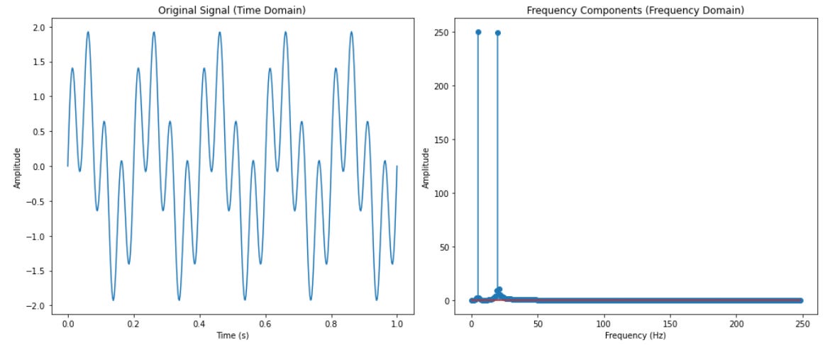
Use Case in AI: Fourier transforms are crucial in signal processing, as they break down complex signals into their individual frequency components using trigonometric functions like sine and cosine. This decomposition technique is widely applied in fields such as audio processing, speech recognition, and time-series analysis, enabling models to identify patterns, frequencies, and trends within data. Although the Fourier Transform primarily uses sine and cosine functions, rather than their reciprocals (cosecant and secant), these foundational trigonometric functions are integral to the process, making Fourier analysis essential for applications where frequency insights are key.
Applications:
- Audio Signal Processing: Fourier transforms help analyze sound waves by decomposing them into sine and cosine components, useful for voice recognition and sound classification tasks.
- Time-Series Analysis in Predictive Modeling: Fourier transforms help analyze periodic patterns and trends in time-series data, useful for predicting seasonality and identifying anomalies.

Here’s a Python example demonstrating the Fourier Transform in signal processing. We’ll use the Fourier Transform to analyze a composite signal made of multiple sine waves, focusing on frequency decomposition.

import numpy as np
import matplotlib.pyplot as plt

# Generate a sample signal composed of two sine waves (5 Hz and 20 Hz frequencies)
t = np.linspace(0, 1, 500)  # Time vector from 0 to 1 second with 500 points
signal = np.sin(2 * np.pi * 5 * t) + np.sin(2 * np.pi * 20 * t)  # Composite signal

# Perform Fourier Transform on the signal
freq_components = np.fft.fft(signal)

# Calculate frequency values (frequency bins)
frequencies = np.fft.fftfreq(len(signal), d=t[1] - t[0])

# Plot the original signal
plt.figure(figsize=(14, 6))
plt.subplot(1, 2, 1)
plt.plot(t, signal)
plt.title("Original Signal (Time Domain)")
plt.xlabel("Time (s)")
plt.ylabel("Amplitude")

# Plot the magnitude of the Fourier Transform (Frequency Domain)
plt.subplot(1, 2, 2)
plt.stem(frequencies[:len(frequencies) // 2], np.abs(freq_components)[:len(frequencies) // 2], use_line_collection=True)
plt.title("Frequency Components (Frequency Domain)")
plt.xlabel("Frequency (Hz)")
plt.ylabel("Amplitude")

plt.tight_layout()
plt.show()

4. Secant (sec): 3D Projections in Computer Vision and Augmented Reality

Use Case in AI: Secant functions are used in 3D projections and transformations in augmented reality (AR) and computer vision. These functions help render objects at different scales or perspectives based on the viewer’s position.
Applications:
- Augmented Reality (AR): Secant functions assist in calculating scaling factors for objects to appear proportionally realistic in AR applications.
- Camera Calibration and Distortion Correction: For cameras that introduce distortion, secant functions can adjust and calibrate these distortions, making images appear more realistic.

import math

# Define the angle in degrees
angle_degrees = 45
angle_radians = math.radians(angle_degrees)

# Calculate secant (1 / cos(angle))
secant = 1 / math.cos(angle_radians)
print(f"Secant of {angle_degrees} degrees: {secant:.2f}")

5. Cotangent (cot): Gradient Calculation in Loss Function Analysis

Use Case in AI: The cotangent function is helpful in advanced loss function analysis and optimization. By examining the cotangent of gradient angles, algorithms can fine-tune adjustments based on the steepness of gradients.
Applications:
- Backpropagation in Neural Networks: Cotangent can assist in adjusting learning rates by examining the gradient’s steepness, improving weight adjustments during backpropagation.
- Recurrent Neural Networks (RNNs): In gradient-based optimization, cotangent helps address gradient vanishing issues, common in RNNs for long sequence processing.

import math

# Define the angle in degrees
angle_degrees = 45
angle_radians = math.radians(angle_degrees)

# Calculate cotangent (1 / tan(angle))
cotangent = 1 / math.tan(angle_radians)
print(f"Cotangent of {angle_degrees} degrees: {cotangent:.2f}")

Conclusion

These trigonometric ratios provide essential mathematical tools for managing rotations, projections, signal decomposition, and optimization in AI. By applying sine, cosine, tangent, and their reciprocals, AI models can handle complex spatial and geometric transformations, analyze signals, and optimize learning processes. Such applications are particularly crucial in fields requiring a strong understanding of geometry, such as computer vision, robotics, and neural network training.

Stay Curious! Share the Knowledge

Thank you for diving into the world of trigonometry in AI with me! If you found this article insightful, please share it with others who are passionate about AI and machine learning. For more content on AI applications, math in data science, and Python coding examples, follow my blog and connect with me on LinkedIn. Let's keep exploring the fascinating ways math powers technology!

For more in-depth technical insights and articles, feel free to explore:

LinkTree: LinkTree - Ebasiq
Substack: ebasiq by Girish
YouTube Channel: Ebasiq YouTube Channel
Instagram: Ebasiq Instagram
Technical Blog: Ebasiq Blog
GitHub Code Repository: Girish GitHub Repos
LinkedIn: Girish LinkedIn

ebasiq by Girish