Overfitting vs Underfitting in ML Models: Balancing Model Complexity for Better Predictions

Striking the Right Balance: Avoiding Underfitting and Overfitting for Accurate Predictions

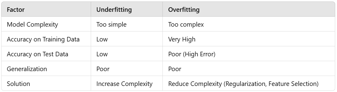
1. Understanding Overfitting and Underfitting

• Underfitting occurs when the model is too simple and cannot capture the underlying patterns in the data.

• Overfitting happens when the model is too complex and learns noise along with the actual pattern in the training data.

Understanding Noise in Overfitting

Noise refers to irrelevant, random, or unnecessary details in the data that do not contribute to the actual patterns we want to learn. When a model overfits, it learns this noise along with the actual trend, making it perform poorly on new data.

Face Recognition Example

• Noise = Background, lighting conditions, hairstyle, or accessories

• An overfitted model might memorize specific features of training images, like a red background or a specific lighting condition.

• If the person is wearing glasses or is in a different lighting environment, the model might fail to recognize them.

Example of Noise

• The model learns: “This is John because he has a blue background and a specific hairstyle.”

• When John changes his hairstyle or takes a photo outside, the model fails to recognize him because it relied on unimportant details.

Exam Preparation Example

• Noise = Exact numbers in practice questions

• In overfitting, you memorize previous exam answers instead of understanding concepts.

• If the question changes slightly, you fail because you relied on specific numbers rather than the method to solve them.

Example of Noise

• Memorizing: “5+3 = 8, 7+2 = 9” instead of learning how to add numbers in general.

• When the question changes to 6+4 = ?, you struggle because you only memorized past answers, not the method.

How to Avoid Learning Noise in Overfitting?

1. Use More Generalized Data → Train models (or humans!) on diverse examples.

2. Reduce Complexity → Don’t make the model too complex, which forces it to learn everything, even unnecessary details.

3. Apply Regularization (for ML models) → Prevent models from giving too much importance to noise.

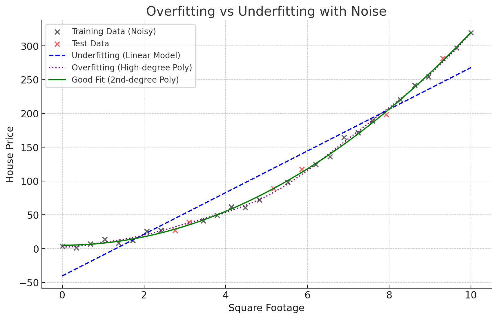
Explanation of the Plot

• Black & Red Dots (Data Points): These represent real-world noisy data (house prices vs square footage).

• Blue Line (Underfitting - Linear Model):

  • Too simple and doesn't capture the underlying pattern.

  • Problem: The model ignores important trends in the data.

• Purple Dotted Line (Overfitting - High-Degree Polynomial):

  • Too complex and captures even the noise in training data.

  • Problem: The model memorizes unnecessary details, failing on new data.

• Green Line (Good Fit - 2nd Degree Polynomial):

  • Captures the real pattern while ignoring noise.

  • ✅ Best model for real-world predictions.

Key Takeaways

1. Overfitting happens when the model learns unnecessary noise.

   • (Purple Dotted Line: It follows every tiny variation in data.)

2. Underfitting happens when the model is too simple.

   • (Blue Line: It doesn't capture the overall trend.)

3. The right balance is needed to generalize well.

   • (Green Line: It follows the true pattern while ignoring noise.)

2. Python Example: Overfitting vs Underfitting

import numpy as np
import matplotlib.pyplot as plt
from sklearn.linear_model import LinearRegression
from sklearn.preprocessing import PolynomialFeatures
from sklearn.metrics import mean_squared_error

# Generate some synthetic data (real-world use case: predicting house prices based on square footage)
np.random.seed(42)
X = np.linspace(1, 10, 20).reshape(-1, 1)  # Features (e.g., Square footage of a house)
y = 3 * X**2 + 2*X + 1 + np.random.normal(0, 5, size=X.shape)  # Non-linear relationship with noise

# Split into training and test set
X_train, X_test = X[:15], X[15:]
y_train, y_test = y[:15], y[15:]

# Underfitting (Linear Regression)
linear_model = LinearRegression()
linear_model.fit(X_train, y_train)
y_pred_linear = linear_model.predict(X_test)

# Overfitting (High-degree Polynomial Regression)
poly_features = PolynomialFeatures(degree=10)
X_poly_train = poly_features.fit_transform(X_train)
X_poly_test = poly_features.transform(X_test)

poly_model = LinearRegression()
poly_model.fit(X_poly_train, y_train)
y_pred_poly = poly_model.predict(X_poly_test)

# True pattern (3rd-degree polynomial for optimal balance)
poly_features_optimal = PolynomialFeatures(degree=2)
X_poly_train_opt = poly_features_optimal.fit_transform(X_train)
X_poly_test_opt = poly_features_optimal.transform(X_test)

optimal_model = LinearRegression()
optimal_model.fit(X_poly_train_opt, y_train)
y_pred_optimal = optimal_model.predict(X_test)

# Plot results
plt.scatter(X_test, y_test, color='black', label="Actual Data")
plt.plot(X_test, y_pred_linear, label="Underfitting (Linear Model)", linestyle='dashed', color='red')
plt.plot(X_test, y_pred_poly, label="Overfitting (High-degree Poly)", linestyle='dotted', color='blue')
plt.plot(X_test, y_pred_optimal, label="Optimal Model (2nd-degree Poly)", color='green')
plt.legend()
plt.xlabel("Square Footage")
plt.ylabel("House Price")
plt.title("Overfitting vs Underfitting")
plt.show()

# Print Mean Squared Errors
print("MSE (Underfitting - Linear Regression):", mean_squared_error(y_test, y_pred_linear))
print("MSE (Overfitting - High-degree Polynomial Regression):", mean_squared_error(y_test, y_pred_poly))
print("MSE (Optimal - 2nd-degree Polynomial Regression):", mean_squared_error(y_test, y_pred_optimal))

3. Real-world Use Cases of Overfitting vs Underfitting

(1) Stock Market Prediction

• Underfitting: If you only use linear regression for stock prices, you might miss complex patterns.

• Overfitting: If you fit a very high-degree polynomial, the model may capture noise in the stock market rather than real trends.

• Balanced Approach: Use techniques like regularization (Lasso/Ridge Regression) or moving averages for better generalization.

(2) Medical Diagnosis

• Underfitting: A simple logistic regression model may fail to capture the non-linear relationships between symptoms and diseases.

• Overfitting: A deep neural network trained with too many parameters might memorize training data rather than learning true patterns.

• Balanced Approach: Use a well-tuned Decision Tree or an ensemble model like Random Forest.

(3) Fraud Detection in Banking

• Underfitting: A model with only basic transaction features (amount, time) might fail to detect fraud.

• Overfitting: A model that includes too many engineered features might learn patterns that are not relevant to fraud.

• Balanced Approach: Feature selection, cross-validation, and using XGBoost or Random Forest can provide a good trade-off.

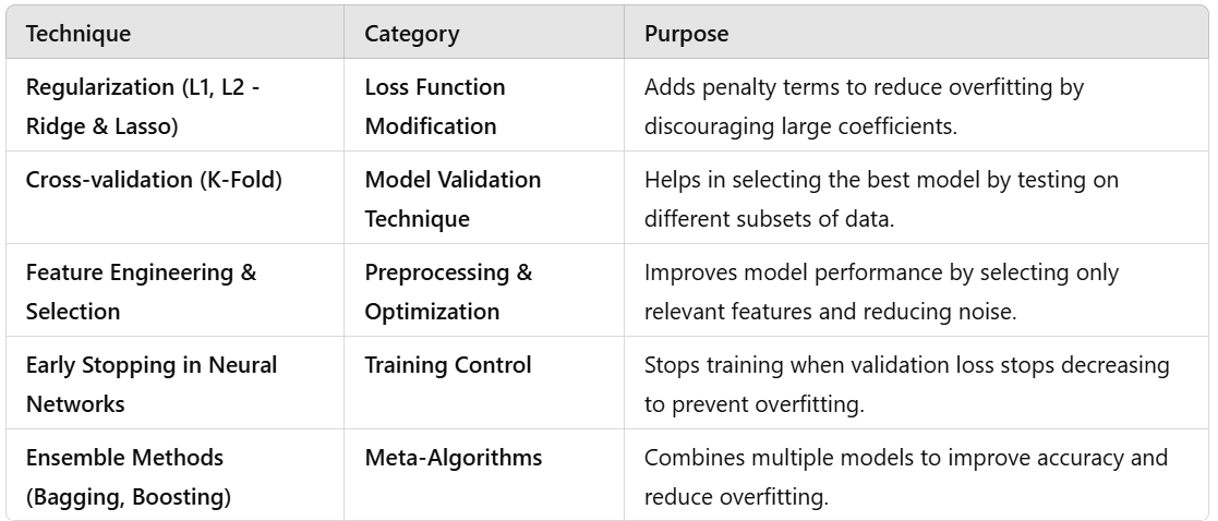
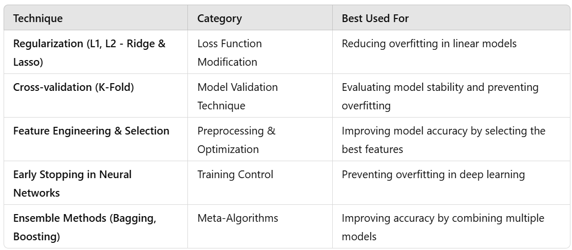
4. How to Avoid Overfitting and Underfitting

• Regularization (L1, L2 - Ridge & Lasso)

• Cross-validation (K-Fold)

• Feature Engineering & Selection

• Early Stopping in Neural Networks

• Ensemble Methods (Bagging, Boosting)

How to Avoid Overfitting and Underfitting - Classification of Techniques

1. Regularization (L1, L2 - Ridge & Lasso)

• Category: Loss Function Modification

• What it does: Adds a penalty to the loss function to prevent the model from giving too much importance to certain features.

• Types:

  • L1 Regularization (Lasso Regression): Shrinks some feature weights to zero (performs feature selection).

  • L2 Regularization (Ridge Regression): Penalizes large weights but does not shrink them to zero.

• Example in Python (Ridge Regression)

from sklearn.linear_model import Ridge

ridge_model = Ridge(alpha=1.0)  # Alpha is the regularization strength
ridge_model.fit(X_train, y_train)

2. Cross-validation (K-Fold)

• Category: Model Validation Technique

• What it does: Splits data into multiple training and test sets (folds) to evaluate model performance on different parts of the data.

• Example in Python

from sklearn.model_selection import cross_val_score
from sklearn.linear_model import LinearRegression

model = LinearRegression()
scores = cross_val_score(model, X, y, cv=5)  # 5-fold cross-validation
print("Cross-validation scores:", scores)

3. Feature Engineering & Selection

• Category: Preprocessing & Optimization

• What it does: Identifies and selects the most relevant features, removing redundant or noisy data.

• Techniques:

  • Removing highly correlated features

  • Using domain knowledge to select important features

  • Applying PCA (Principal Component Analysis)

• Example in Python (Feature Selection using Correlation)

import pandas as pd

# Assume df is a DataFrame with features and target variable
correlation_matrix = df.corr()
print(correlation_matrix["target"].sort_values(ascending=False))  # Checking correlation with target

4. Early Stopping in Neural Networks

• Category: Training Control

• What it does: Stops training when validation loss no longer decreases to avoid overfitting.

• Example in Python (Using TensorFlow/Keras)

from tensorflow.keras.callbacks import EarlyStopping

early_stopping = EarlyStopping(monitor='val_loss', patience=5, restore_best_weights=True)

model.fit(X_train, y_train, validation_data=(X_val, y_val), epochs=100, callbacks=[early_stopping])

5. Ensemble Methods (Bagging, Boosting)

• Category: Meta-Algorithms

• What it does: Combines multiple models to improve predictions.

• Types:

  • Bagging (Bootstrap Aggregating): Trains multiple models on random subsets of data and averages the results (e.g., Random Forest).

  • Boosting: Sequentially trains models, giving more weight to errors (e.g., XGBoost, AdaBoost).

• Example in Python (Random Forest - Bagging)

from sklearn.ensemble import RandomForestRegressor

rf_model = RandomForestRegressor(n_estimators=100, random_state=42)
rf_model.fit(X_train, y_train)

Summary

FAQ’s

1. What is a Loss Function?

A Loss Function is like a teacher’s feedback in Machine Learning. It tells your model how wrong its predictions are and helps it improve during training.

Simple Example: Learning to Throw a Basketball

Imagine you're learning to shoot a basketball into a hoop.

1. You take a shot...

2. You miss the hoop by 2 feet. ❌

3. You adjust your aim and try again.

4. You keep practicing until you consistently score! ✅

👉 Here, “how far you missed the hoop” is the Loss Function. It measures the mistake and guides you to improve your aim.

Loss Function in Machine Learning

In ML, a model makes predictions (like shooting the basketball).

• The Loss Function calculates how far the prediction is from the actual answer (just like measuring how far the ball missed the hoop).

• The model then adjusts itself (like you correcting your aim) to minimize this loss.

Real-life Example: Predicting House Prices 🏡

Let’s say you're building a model to predict house prices.

👉 The Loss Function tells us how far the predicted price is from the actual price.
👉 The model then adjusts itself (like learning from mistakes) to reduce this error.

Types of Loss Functions

🔹 Mean Squared Error (MSE) ⚡ – Used for regression (predicting continuous values).
🔹 Cross-Entropy Loss 🔥 – Used for classification (predicting categories like spam/not spam).

Explanation of the Loss Function Example

We calculated two different loss functions for regression and classification problems.

1️⃣ Regression (Mean Squared Error - MSE)

• Real-life case: Predicting house prices.

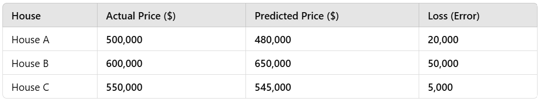
• Actual vs. Predicted Prices:

  • House A: 500K (Actual) vs. 480K (Predicted)

  • House B: 600K (Actual) vs. 650K (Predicted)

  • House C: 550K (Actual) vs. 545K (Predicted)

• MSE Loss: 975.00 (Higher value means bigger errors).

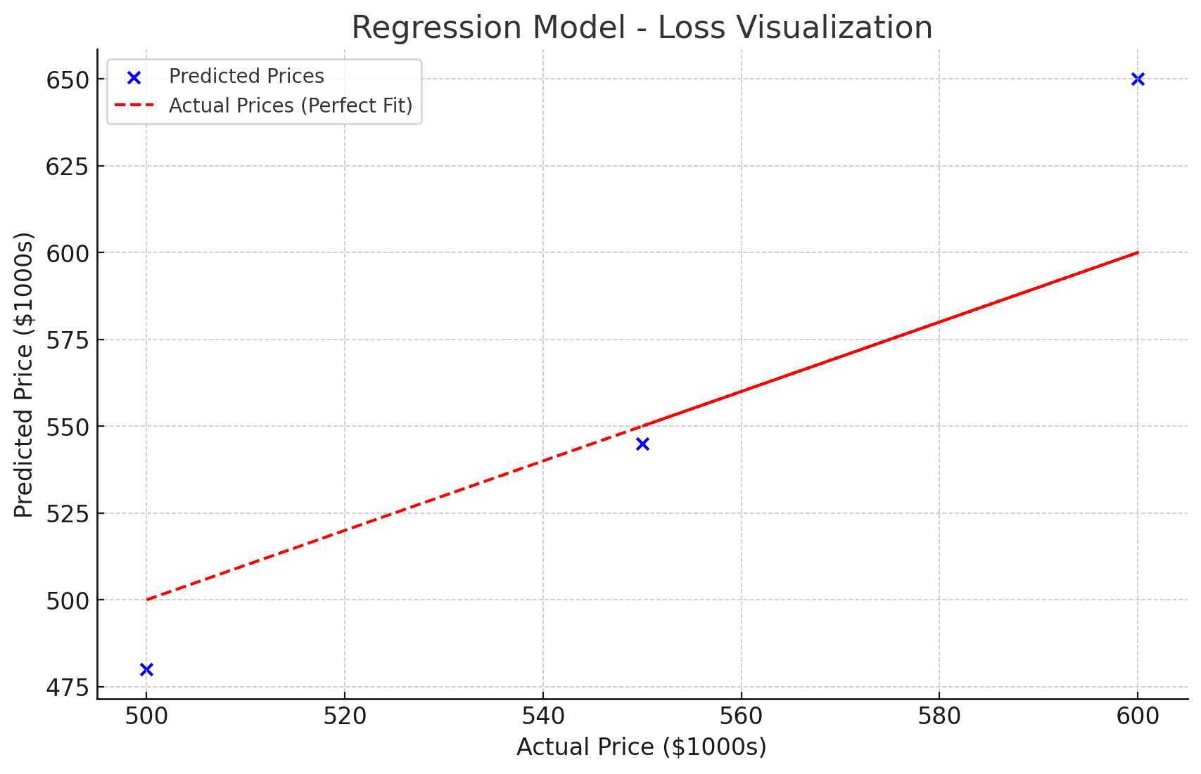
Visualization:

• 🔵 Blue points → Model’s predictions.

• 🔴 Red dashed line → Perfect predictions (ideal case).

• More deviation from the red line = Higher loss.

2️⃣ Classification (Cross-Entropy Loss)

• Real-life case: Predicting whether an email is spam.

• Actual vs. Predicted Probabilities:

  • Email 1: Spam (1) → Predicted 0.9 (90%)

  • Email 2: Not Spam (0) → Predicted 0.1 (10%)

  • Email 3: Spam (1) → Predicted 0.4 (40%) ❌

  • Email 4: Not Spam (0) → Predicted 0.6 (60%) ❌

• Cross-Entropy Loss: 0.51 (Lower is better).

📌 Meaning of Cross-Entropy Loss:

• When the model predicts with high confidence and is correct, loss is low. ✅

• When the model makes wrong predictions, loss is high. ❌

Summary

✅ Loss functions measure how wrong a model’s predictions are.
✅ Lower loss means better performance.
✅ Different loss functions are used for different tasks:

• MSE for Regression (predicting numbers).

• Cross-Entropy for Classification (predicting categories like spam/not spam).

2. What is Bagging vs. Boosting?

Bagging and Boosting are two popular techniques used to improve the accuracy and stability of machine learning models. They both fall under the category of ensemble learning, where multiple models are combined to make better predictions.

Think of them like a group of students working on an exam:

• Bagging: Everyone solves the same exam separately, and we combine their answers to get the best solution.

• Boosting: Each student learns from the mistakes of the previous student, improving step by step.

1️⃣ Bagging (Bootstrap Aggregating)

Definition

Bagging is a technique where multiple models (usually decision trees) are trained independently on different random subsets of the data, and their predictions are averaged (for regression) or voted (for classification).

Real-Life Example: Who Wants to Be a Millionaire? (Audience Poll 📊)

Imagine you're on the game show "Who Wants to Be a Millionaire?" and you're unsure about the answer to a question. You use the Audience Poll lifeline:

• Each audience member gives their own independent answer.

• The final answer is the most popular choice.

✅ Why it works: Even if some audience members are wrong, the majority vote is likely correct!

How Bagging Works (Steps)

1. Randomly select multiple subsets of the training data (with replacement).

2. Train several weak models (e.g., decision trees) independently.

3. Aggregate their predictions:

   • Regression: Take the average of all predictions.

   • Classification: Use majority voting (the most common answer wins).

🔹 Example Algorithm: Random Forest (Bagging Applied to Decision Trees)

Random Forest is a famous algorithm that uses bagging to train multiple decision trees and combine their outputs.

2️⃣ Boosting (Sequential Learning)

Definition

Boosting is a technique where models are trained sequentially, and each new model focuses on fixing the mistakes of the previous model.

Real-Life Example: Teaching a Kid to Ride a Bicycle 🚲

Imagine you're teaching a child how to ride a bike:

1. First attempt: They fall off. ❌

2. Second attempt: You help them balance better. ✅

3. Third attempt: They now struggle with turning, so you guide them on that. ✅

4. Final attempt: They ride successfully! 🎉

✅ Why it works: Each time, you correct the previous mistake, so the child learns progressively better.

How Boosting Works (Steps)

1. Train a simple model (e.g., a small decision tree).

2. Find where it makes mistakes and give those errors more importance.

3. Train the next model to focus on these difficult examples.

4. Repeat this process multiple times.

5. Combine all models’ outputs for final prediction.

🔹 Example Algorithms:

• AdaBoost (Adaptive Boosting)

• Gradient Boosting (GBM)

• XGBoost (Extreme Gradient Boosting)

• LightGBM (Light Gradient Boosting Machine)

Python Code Example

Let’s see Bagging vs Boosting in action using Random Forest (Bagging) and AdaBoost (Boosting).

from sklearn.ensemble import RandomForestClassifier, AdaBoostClassifier
from sklearn.datasets import make_classification
from sklearn.model_selection import train_test_split
from sklearn.metrics import accuracy_score

# Generate a synthetic dataset
X, y = make_classification(n_samples=1000, n_features=20, random_state=42)

# Split into training and test sets
X_train, X_test, y_train, y_test = train_test_split(X, y, test_size=0.2, random_state=42)

# Bagging: Random Forest (Multiple Decision Trees)
bagging_model = RandomForestClassifier(n_estimators=50, random_state=42)
bagging_model.fit(X_train, y_train)
y_pred_bagging = bagging_model.predict(X_test)

# Boosting: AdaBoost (Sequential Weak Learners)
boosting_model = AdaBoostClassifier(n_estimators=50, random_state=42)
boosting_model.fit(X_train, y_train)
y_pred_boosting = boosting_model.predict(X_test)

# Evaluate Performance
accuracy_bagging = accuracy_score(y_test, y_pred_bagging)
accuracy_boosting = accuracy_score(y_test, y_pred_boosting)

print(f"Bagging (Random Forest) Accuracy: {accuracy_bagging:.2f}")
print(f"Boosting (AdaBoost) Accuracy: {accuracy_boosting:.2f}")

• Use Bagging when your model is overfitting (reduces variance).

• Use Boosting when your model is underfitting (reduces bias).

• Random Forest (Bagging) is best for stability and generalization.

• XGBoost (Boosting) is best for handling complex patterns.

Conclusion

Understanding the difference between underfitting and overfitting is crucial for building machine learning models that generalize well to real-world data. A well-balanced model learns the true underlying patterns while ignoring unnecessary noise, leading to better accuracy and reliability.

Key Takeaways:
✅ Underfitting → Model is too simple, fails to learn.
✅ Overfitting → Model is too complex, learns unnecessary noise.
✅ Balanced Model → Captures patterns without memorizing noise.

🔥 Want to dive deeper? Try experimenting with regularization, cross-validation, and ensemble methods to fine-tune your models!

👉 Have you encountered overfitting or underfitting in your projects? Share your experiences in the comments! 🚀

---

For more in-depth technical insights and articles, feel free to explore:

Girish Central

• LinkTree: GirishHub – A single hub for all my content, resources, and online presence.

• LinkedIn: Girish LinkedIn – Connect with me for professional insights, updates, and networking.

Ebasiq

• Substack: ebasiq by Girish – In-depth articles on AI, Python, and technology trends.

• Technical Blog: Ebasiq Blog – Dive into technical guides and coding tutorials.

• GitHub Code Repository: Girish GitHub Repos – Access practical Python, AI/ML, Full Stack and coding examples.

• YouTube Channel: Ebasiq YouTube Channel – Watch tutorials and tech videos to enhance your skills.

• Instagram: Ebasiq Instagram – Follow for quick tips, updates, and engaging tech content.

GirishBlogBox

• Substack: Girish BlogBlox – Thought-provoking articles and personal reflections.

• Personal Blog: Girish - BlogBox – A mix of personal stories, experiences, and insights.

Ganitham Guru

• Substack: Ganitham Guru – Explore the beauty of Vedic mathematics, Ancient Mathematics, Modern Mathematics and beyond.

• Mathematics Blog: Ganitham Guru – Simplified mathematics concepts and tips for learners.