Mastering Deep CNN Challenges with ResNet: A Comprehensive Guide

Solving Deep Learning Challenges with Residual Networks: A Complete Guide to CNN Limitations, ResNet Variants, and Practical Transfer Learning Using TensorFlow

Apr 17, 2025

1. Introduction: Why Depth Isn’t Always Better

Over the past decade, deeper Convolutional Neural Networks (CNNs) have significantly improved performance in computer vision tasks. From AlexNet to VGG and beyond, stacking more layers seemed to yield better results. However, researchers encountered a surprising problem: beyond a certain depth, adding more layers made models worse—not better.

The Intuition:

A deeper model should, in theory, be better since it can represent more complex functions. But, in practice, it begins to:

Train slower or not at all.
Perform worse on the test set.
Lose its learning ability.

Why This Happens?

Because of issues like:

Vanishing gradients
Training instability
Overfitting
Degradation in accuracy

This guide walks you through these challenges and the powerful solution: ResNet (Residual Networks).

2. Challenges with CNNs

CNNs are brilliant at extracting features. But as depth increases, several practical problems surface.

Key Issues:

Vanishing Gradient Problem
- The gradients become extremely small as they are backpropagated through many layers.
- Early layers stop learning.
Degradation Problem
- Accuracy decreases as layers are added (even when the added layers should theoretically help).
Overfitting in Small Datasets
- Deep CNNs tend to memorize instead of generalizing, especially when training data is limited.
Optimization Difficulty
- Deep models become harder to train, requiring very careful initialization and tuning.
Computational Cost
- More layers = more parameters = higher memory and processing needs.

Analogy:

Think of CNNs like a production line. Each layer is a worker. As you keep adding more workers, miscommunication or fatigue sets in, and instead of improving efficiency, things slow down or break.

3. The Vanishing Gradient Problem (with Analogy)

What is it?

In deep networks, during backpropagation, gradients (which tell the model how to update weights) become tiny. This is especially true when using sigmoid or tanh activations.

What’s the Impact?

Early layers barely receive updates.
Network training stagnates.
Accuracy plateaus or degrades.

Technical Insight:

If each layer’s gradient is 0.9, after 50 layers:
Gradient ≈ 0.9^50 ≈ 0.005 → negligible!

Analogy:

Imagine whispering a message down a long line of people. The original message becomes so faint or garbled that the person at the beginning hears nothing useful.

4. Batch Normalization: A Stepping Stone Solution

What is it?

Batch Normalization (BatchNorm) normalizes the input of each layer to have a mean ≈ 0 and standard deviation ≈ 1. This helps stabilize and speed up training.

How It Works:

For each mini-batch, it:

Calculates mean and variance.
Normalizes each feature.
Applies scale (γ) and shift (β) parameters (which are trainable).

Benefits:

Reduces internal covariate shift.
Allows higher learning rates.
Improves gradient flow.
Acts as a regularizer.

Example:

x = layers.Conv2D(64, 3, padding='same')(input)
x = layers.BatchNormalization()(x)
x = layers.ReLU()(x)

Analogy:

It’s like giving every student the same energy drink before a race. Everyone starts with a similar energy level, making the race fair and consistent.

5. ResNet: The Residual Learning Breakthrough

Key Idea:

Instead of directly learning H(x), ResNet learns F(x) = H(x) - x. Then it adds the input back:

Output: H(x)=F(x)+x

This is called a skip connection or shortcut connection.

What It Does:

Allows the gradient to flow directly.
Preserves the original input signal.
Solves the vanishing gradient problem.
Trains very deep networks (100+ layers) effectively.

Real-World Applications:

Medical Imaging – Tumor classification
Self-Driving Cars – Object detection, lane recognition
Face Recognition – Used in FaceNet, ArcFace
Video Surveillance – Person re-identification
Industry – Defect detection, quality control

Visual:

Input → [Conv → BN → ReLU → Conv → BN] → Add(Input) → ReLU → Output

6. Types of ResNet Architectures (with Comparison Table)

ResNet comes in several variants depending on depth and block structure.

Two Major Block Types:

ResNet Model Comparison Table

Mini ResNet

A simplified ResNet with fewer blocks.
Great for educational purposes or mobile devices.

7. Mini ResNet Example + Training + Prediction

import tensorflow as tf
from tensorflow.keras import layers, models

def mini_residual_block(x):
    shortcut = x
    x = layers.Conv2D(32, 3, padding='same', activation='relu')(x)
    x = layers.Conv2D(32, 3, padding='same')(x)
    x = layers.Add()([x, shortcut])
    return layers.Activation('relu')(x)

def mini_resnet(input_shape=(32, 32, 3), num_classes=10):
    inputs = layers.Input(shape=input_shape)
    x = layers.Conv2D(32, 3, padding='same', activation='relu')(inputs)
    x = mini_residual_block(x)
    x = layers.GlobalAveragePooling2D()(x)
    outputs = layers.Dense(num_classes, activation='softmax')(x)
    return models.Model(inputs, outputs)

# Load and preprocess data
(x_train, y_train), (x_test, y_test) = tf.keras.datasets.cifar10.load_data()
x_train, x_test = x_train / 255.0, x_test / 255.0

model = mini_resnet()
model.compile(optimizer='adam', loss='sparse_categorical_crossentropy', metrics=['accuracy'])

# Train model (optional: just 1 epoch for demo)
model.fit(x_train, y_train, epochs=1, batch_size=64, validation_split=0.1)

# Predict
import numpy as np
pred = model.predict(np.expand_dims(x_test[0], axis=0))
print("Prediction:", tf.argmax(pred[0]).numpy())

8. ResNet-18 and ResNet-34: Hands-On with Residual Blocks

Basic Residual Block Code:

def resnet_basic_block(x, filters, stride=1):
    shortcut = x
    x = layers.Conv2D(filters, 3, strides=stride, padding='same', use_bias=False)(x)
    x = layers.BatchNormalization()(x)
    x = layers.ReLU()(x)
    x = layers.Conv2D(filters, 3, padding='same', use_bias=False)(x)
    x = layers.BatchNormalization()(x)

    if stride != 1 or shortcut.shape[-1] != filters:
        shortcut = layers.Conv2D(filters, 1, strides=stride, use_bias=False)(shortcut)
        shortcut = layers.BatchNormalization()(shortcut)

    x = layers.Add()([x, shortcut])
    return layers.ReLU()(x)

Model Builder:

def build_resnet(input_shape, num_classes, layers_per_stage):
    inputs = layers.Input(shape=input_shape)
    x = layers.Conv2D(64, 3, padding='same', use_bias=False)(inputs)
    x = layers.BatchNormalization()(x)
    x = layers.ReLU()(x)

    filters = 64
    for stage, num_blocks in enumerate(layers_per_stage):
        for block in range(num_blocks):
            stride = 2 if block == 0 and stage != 0 else 1
            x = resnet_basic_block(x, filters, stride)
        filters *= 2

    x = layers.GlobalAveragePooling2D()(x)
    outputs = layers.Dense(num_classes, activation='softmax')(x)
    return models.Model(inputs, outputs)

# Example for ResNet-18 and ResNet-34
resnet18 = build_resnet((32, 32, 3), 10, [2, 2, 2, 2])
resnet34 = build_resnet((32, 32, 3), 10, [3, 4, 6, 3])

9. ResNet-50, 101, 152: Bottleneck Blocks and Bigger Networks

Bottleneck Block:

def resnet_bottleneck_block(x, filters, stride=1):
    shortcut = x

    x = layers.Conv2D(filters, 1, strides=stride, padding='same', use_bias=False)(x)
    x = layers.BatchNormalization()(x)
    x = layers.ReLU()(x)

    x = layers.Conv2D(filters, 3, padding='same', use_bias=False)(x)
    x = layers.BatchNormalization()(x)
    x = layers.ReLU()(x)

    x = layers.Conv2D(filters * 4, 1, padding='same', use_bias=False)(x)
    x = layers.BatchNormalization()(x)

    if stride != 1 or shortcut.shape[-1] != filters * 4:
        shortcut = layers.Conv2D(filters * 4, 1, strides=stride, use_bias=False)(shortcut)
        shortcut = layers.BatchNormalization()(shortcut)

    x = layers.Add()([x, shortcut])
    return layers.ReLU()(x)

Bottleneck ResNet Builder:

def build_resnet_bottleneck(input_shape, num_classes, layers_per_stage):
    inputs = layers.Input(shape=input_shape)
    x = layers.Conv2D(64, 7, strides=2, padding='same', use_bias=False)(inputs)
    x = layers.BatchNormalization()(x)
    x = layers.ReLU()(x)
    x = layers.MaxPooling2D(3, strides=2, padding='same')(x)

    filters = 64
    for stage, num_blocks in enumerate(layers_per_stage):
        for block in range(num_blocks):
            stride = 2 if block == 0 and stage != 0 else 1
            x = resnet_bottleneck_block(x, filters, stride)
        filters *= 2

    x = layers.GlobalAveragePooling2D()(x)
    outputs = layers.Dense(num_classes, activation='softmax')(x)
    return models.Model(inputs, outputs)

# ResNet-50 / 101 / 152
resnet50 = build_resnet_bottleneck((32, 32, 3), 10, [3, 4, 6, 3])
resnet101 = build_resnet_bottleneck((32, 32, 3), 10, [3, 4, 23, 3])
resnet152 = build_resnet_bottleneck((32, 32, 3), 10, [3, 8, 36, 3])

11. Transfer Learning with ResNet + ImageNet

What is Transfer Learning?

Transfer Learning is a technique where a model trained on one large dataset (like ImageNet) is reused or fine-tuned for a different but related task.

Rather than training a model from scratch, you "transfer" the learned weights and representations to save time, compute, and improve accuracy, especially when your dataset is small.

Why Use Transfer Learning?

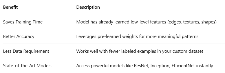
How to Use Pretrained ResNet from ImageNet in TensorFlow

Example: Feature Extraction using ResNet-50

from tensorflow.keras.applications import ResNet50
from tensorflow.keras.layers import GlobalAveragePooling2D, Dense, Input
from tensorflow.keras.models import Model

# Load pretrained ResNet50 base (excluding top layers)
base_model = ResNet50(weights='imagenet', include_top=False, input_shape=(224, 224, 3))
base_model.trainable = False  # Freeze base layers

# Add custom classifier head
inputs = Input(shape=(224, 224, 3))
x = base_model(inputs, training=False)
x = GlobalAveragePooling2D()(x)
x = Dense(256, activation='relu')(x)
outputs = Dense(5, activation='softmax')(x)  # For example, 5 custom classes

model = Model(inputs, outputs)

model.compile(optimizer='adam', loss='sparse_categorical_crossentropy', metrics=['accuracy'])
model.summary()

🔁 This architecture is ideal when you want to use ResNet's feature extraction power, but fine-tune only the classifier part for your own dataset.

Fine-Tuning Deeper Layers (Optional)

If you have more data or want to improve accuracy further:

base_model.trainable = True  # Unfreeze for fine-tuning
# Compile with lower learning rate
model.compile(optimizer=tf.keras.optimizers.Adam(1e-5), loss='sparse_categorical_crossentropy')

Unfreezing and training even part of the ResNet layers can yield better performance — just be careful of overfitting.

Example Use Cases:

Example: Transfer Learning with ResNet50 on CIFAR-10

# Step 1: Import Libraries
import tensorflow as tf
from tensorflow.keras.applications import ResNet50
from tensorflow.keras.applications.resnet50 import preprocess_input
from tensorflow.keras.layers import Input, GlobalAveragePooling2D, Dense
from tensorflow.keras.models import Model
import numpy as np

# Step 2: Load and Preprocess CIFAR-10
(x_train, y_train), (x_test, y_test) = tf.keras.datasets.cifar10.load_data()

# Resize to 224x224 for ResNet50 compatibility
x_train_resized = tf.image.resize(x_train, [224, 224])
x_test_resized = tf.image.resize(x_test, [224, 224])

# Preprocess using ResNet50's preprocessing
x_train_preprocessed = preprocess_input(x_train_resized)
x_test_preprocessed = preprocess_input(x_test_resized)

# Step 3: Create ResNet50 Transfer Learning Model
base_model = ResNet50(weights='imagenet', include_top=False, input_shape=(224, 224, 3))
base_model.trainable = False  # Freeze pretrained weights

inputs = Input(shape=(224, 224, 3))
x = base_model(inputs, training=False)
x = GlobalAveragePooling2D()(x)
x = Dense(256, activation='relu')(x)
outputs = Dense(10, activation='softmax')(x)  # 10 CIFAR classes

model = Model(inputs, outputs)

# Step 4: Compile the Model
model.compile(optimizer='adam',
              loss='sparse_categorical_crossentropy',
              metrics=['accuracy'])

# Step 5: Train the Model
history = model.fit(x_train_preprocessed, y_train,
                    validation_split=0.1,
                    epochs=5,
                    batch_size=64)

# Step 6: Evaluate the Model
test_loss, test_acc = model.evaluate(x_test_preprocessed, y_test)
print(f"Test Accuracy: {test_acc:.4f}")

Optional: Fine-Tune Deeper Layers

Unfreeze the last few layers of ResNet50 to improve accuracy:

# Step 7: Fine-Tune the Last Few Layers
base_model.trainable = True

# Optionally freeze first 100 layers
for layer in base_model.layers[:100]:
    layer.trainable = False

# Compile again with a lower learning rate
model.compile(optimizer=tf.keras.optimizers.Adam(1e-5),
              loss='sparse_categorical_crossentropy',
              metrics=['accuracy'])

# Retrain
model.fit(x_train_preprocessed, y_train, validation_split=0.1, epochs=3, batch_size=64)

Use Case: Custom Dataset with ResNet50 (TensorFlow/Keras)

Folder Structure Example:

dataset/
├── train/
│   ├── cats/
│   └── dogs/
├── validation/
│   ├── cats/
│   └── dogs/

# Step 1: Import Libraries
import tensorflow as tf
from tensorflow.keras.applications import ResNet50
from tensorflow.keras.applications.resnet50 import preprocess_input
from tensorflow.keras.preprocessing.image import ImageDataGenerator
from tensorflow.keras.layers import GlobalAveragePooling2D, Dense, Input
from tensorflow.keras.models import Model

# Step 2: Set Image Parameters
IMG_SIZE = (224, 224)
BATCH_SIZE = 32
NUM_CLASSES = 2  # Change if more categories

# Step 3: Prepare Image Generators
train_datagen = ImageDataGenerator(preprocessing_function=preprocess_input)
val_datagen = ImageDataGenerator(preprocessing_function=preprocess_input)

train_gen = train_datagen.flow_from_directory(
    'dataset/train',
    target_size=IMG_SIZE,
    batch_size=BATCH_SIZE,
    class_mode='sparse'
)

val_gen = val_datagen.flow_from_directory(
    'dataset/validation',
    target_size=IMG_SIZE,
    batch_size=BATCH_SIZE,
    class_mode='sparse'
)

# Step 4: Build Transfer Learning Model
base_model = ResNet50(weights='imagenet', include_top=False, input_shape=(224, 224, 3))
base_model.trainable = False

inputs = Input(shape=(224, 224, 3))
x = base_model(inputs, training=False)
x = GlobalAveragePooling2D()(x)
x = Dense(256, activation='relu')(x)
outputs = Dense(NUM_CLASSES, activation='softmax')(x)

model = Model(inputs, outputs)

# Step 5: Compile the Model
model.compile(optimizer='adam',
              loss='sparse_categorical_crossentropy',
              metrics=['accuracy'])

# Step 6: Train the Model
model.fit(train_gen, validation_data=val_gen, epochs=5)

# Step 7: Evaluate or Predict
loss, acc = model.evaluate(val_gen)
print(f"Validation Accuracy: {acc:.4f}")

Fine-Tune ResNet50 on Your Custom Dataset

# Step 8: Unfreeze Top Layers of ResNet50
base_model.trainable = True

# Freeze first 100 layers if needed
for layer in base_model.layers[:100]:
    layer.trainable = False

# Re-compile with lower LR
model.compile(optimizer=tf.keras.optimizers.Adam(1e-5),
              loss='sparse_categorical_crossentropy',
              metrics=['accuracy'])

# Fine-tune
model.fit(train_gen, validation_data=val_gen, epochs=3)

Tips for Better Results

Use ImageDataGenerator for augmentation (rotation_range, zoom_range, etc.)
Use EarlyStopping, ReduceLROnPlateau for training stability
Save model:

model.save("resnet50_custom_model.h5")

🔚 Conclusion

In the fast-evolving world of deep learning, depth is power — but with great depth comes great difficulty. Traditional CNNs struggle with vanishing gradients and degraded performance as they grow deeper. ResNet revolutionized this space by introducing residual connections, making it possible to train models with 50, 101, or even 152 layers effectively.

By mastering ResNet architectures and applying transfer learning from models pretrained on ImageNet, you can achieve powerful results even with small datasets and limited resources.

You now have a complete toolkit — from understanding the theory to implementing ResNet-based models on both standard and custom datasets.

Next Steps: Your Learning Journey

Try out ResNet-50 with transfer learning on your own dataset using the code templates provided.
Experiment with fine-tuning to improve accuracy.
Explore other pretrained models like EfficientNet, Inception, or MobileNet.
Dive deeper into ResNeXt, DenseNet, and Vision Transformers if you’re curious about next-gen architectures.

Call to Action

If this guide helped you:

Bookmark or share it with fellow learners and developers.
Subscribe to my Substack for more deep learning guides and notebooks.
Visit my GitHub for hands-on code and projects.
Follow me on LinkedIn for practical AI tips and student-friendly content.
Feel free to DM me if you'd like to take my Deep Learning + TensorFlow Bootcamp — open for both students and professionals!

For more in-depth technical insights and articles, feel free to explore:

Girish Central

LinkTree: GirishHub – A single hub for all my content, resources, and online presence.
LinkedIn: Girish LinkedIn – Connect with me for professional insights, updates, and networking.

Ebasiq

Substack: ebasiq by Girish – In-depth articles on AI, Python, and technology trends.
Technical Blog: Ebasiq Blog – Dive into technical guides and coding tutorials.
GitHub Code Repository: Girish GitHub Repos – Access practical Python, AI/ML, Full Stack and coding examples.
YouTube Channel: Ebasiq YouTube Channel – Watch tutorials and tech videos to enhance your skills.
Instagram: Ebasiq Instagram – Follow for quick tips, updates, and engaging tech content.

GirishBlogBox

Substack: Girish BlogBlox – Thought-provoking articles and personal reflections.
Personal Blog: Girish - BlogBox – A mix of personal stories, experiences, and insights.

Ganitham Guru

Substack: Ganitham Guru – Explore the beauty of Vedic mathematics, Ancient Mathematics, Modern Mathematics and beyond.
Mathematics Blog: Ganitham Guru – Simplified mathematics concepts and tips for learners.

ebasiq by Girish

Mastering Deep CNN Challenges with ResNet: A Comprehensive Guide

Solving Deep Learning Challenges with Residual Networks: A Complete Guide to CNN Limitations, ResNet Variants, and Practical Transfer Learning Using TensorFlow

1. Introduction: Why Depth Isn’t Always Better

The Intuition:

Why This Happens?

2. Challenges with CNNs

Key Issues:

Analogy:

3. The Vanishing Gradient Problem (with Analogy)

What is it?

What’s the Impact?

Technical Insight:

Analogy:

4. Batch Normalization: A Stepping Stone Solution

What is it?

How It Works:

Benefits:

Example:

Analogy:

5. ResNet: The Residual Learning Breakthrough

Key Idea:

What It Does:

Real-World Applications:

Visual:

6. Types of ResNet Architectures (with Comparison Table)

Two Major Block Types:

ResNet Model Comparison Table

Mini ResNet

7. Mini ResNet Example + Training + Prediction

8. ResNet-18 and ResNet-34: Hands-On with Residual Blocks

Basic Residual Block Code:

Model Builder:

9. ResNet-50, 101, 152: Bottleneck Blocks and Bigger Networks

Bottleneck Block:

Bottleneck ResNet Builder:

11. Transfer Learning with ResNet + ImageNet

What is Transfer Learning?

Why Use Transfer Learning?

How to Use Pretrained ResNet from ImageNet in TensorFlow

Example: Feature Extraction using ResNet-50

Fine-Tuning Deeper Layers (Optional)

Example Use Cases:

Example: Transfer Learning with ResNet50 on CIFAR-10

Optional: Fine-Tune Deeper Layers

Use Case: Custom Dataset with ResNet50 (TensorFlow/Keras)

Folder Structure Example:

Fine-Tune ResNet50 on Your Custom Dataset

Tips for Better Results

🔚 Conclusion

Next Steps: Your Learning Journey

Call to Action

For more in-depth technical insights and articles, feel free to explore:

Girish Central

Ebasiq

GirishBlogBox

Ganitham Guru

Discussion about this post