Convolutional Neural Networks (CNNs) Demystified: A Visual and Practical Learning Guide

Step-by-step explanation with real examples, visual animations, architecture diagrams, and practical workflows

What is a CNN?

A Convolutional Neural Network (CNN) is a type of deep learning model mainly used for image classification, object detection, and image recognition.

CNNs work by:

• Automatically extracting features (like edges, shapes) from images

• Reducing the image dimension while preserving important content

• Using these features for classification or other tasks

In Convolutional Neural Networks (CNNs), convolution refers to the mathematical operation that slides a filter (or kernel) over an input (like an image) to produce a feature map. It's a core process used to extract spatial features like edges, textures, patterns, etc., from the input data.

What is Convolution in Simple Terms?

Imagine a flashlight scanning across a room. At each position, it focuses on a small region and gathers information. That’s exactly what a convolution operation does:

• A small matrix (filter or kernel) moves across the image.

• At each position, it performs element-wise multiplication between the filter and the region it covers.

• It sums the results to produce a single value in the output (called the convolved feature or feature map).

Why Convolution?

It helps the model focus on important features like:

• Edges (vertical, horizontal)

• Corners

• Textures

• Repeated patterns

This process helps the network learn hierarchical features, going from low-level (edges) to high-level (object parts or full objects) as we go deeper.

Real-world Applications of CNN:

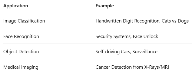
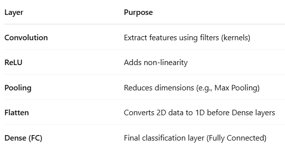
Key Components of a CNN:

Step-by-Step Code: Simple CNN using Keras

import tensorflow as tf
from tensorflow.keras import layers, models
from tensorflow.keras.datasets import mnist
from tensorflow.keras.utils import to_categorical

# Step 1: Load Data
(X_train, y_train), (X_test, y_test) = mnist.load_data()

# Step 2: Preprocess Data
X_train = X_train.reshape((X_train.shape[0], 28, 28, 1)) / 255.0
X_test = X_test.reshape((X_test.shape[0], 28, 28, 1)) / 255.0
y_train = to_categorical(y_train)
y_test = to_categorical(y_test)

# Step 3: Build CNN Model
model = models.Sequential([
    layers.Conv2D(32, (3, 3), activation='relu', input_shape=(28, 28, 1)),  # Convolution
    layers.MaxPooling2D((2, 2)),  # Pooling
    layers.Conv2D(64, (3, 3), activation='relu'),  # Another Conv
    layers.MaxPooling2D((2, 2)),  # Another Pooling
    layers.Flatten(),  # Flatten before FC
    layers.Dense(64, activation='relu'),  # Fully Connected
    layers.Dense(10, activation='softmax')  # Output layer for 10 classes
])

# Step 4: Compile the Model
model.compile(optimizer='adam',
              loss='categorical_crossentropy',
              metrics=['accuracy'])

# Step 5: Train the Model
model.fit(X_train, y_train, epochs=5, batch_size=64, validation_split=0.1)

# Step 6: Evaluate the Model
test_loss, test_acc = model.evaluate(X_test, y_test)
print(f"Test Accuracy: {test_acc:.2f}")

CNN Model - Step-by-Step Flow:

This sequence explains how an input image passes through various layers of a Convolutional Neural Network (CNN) for prediction.

---

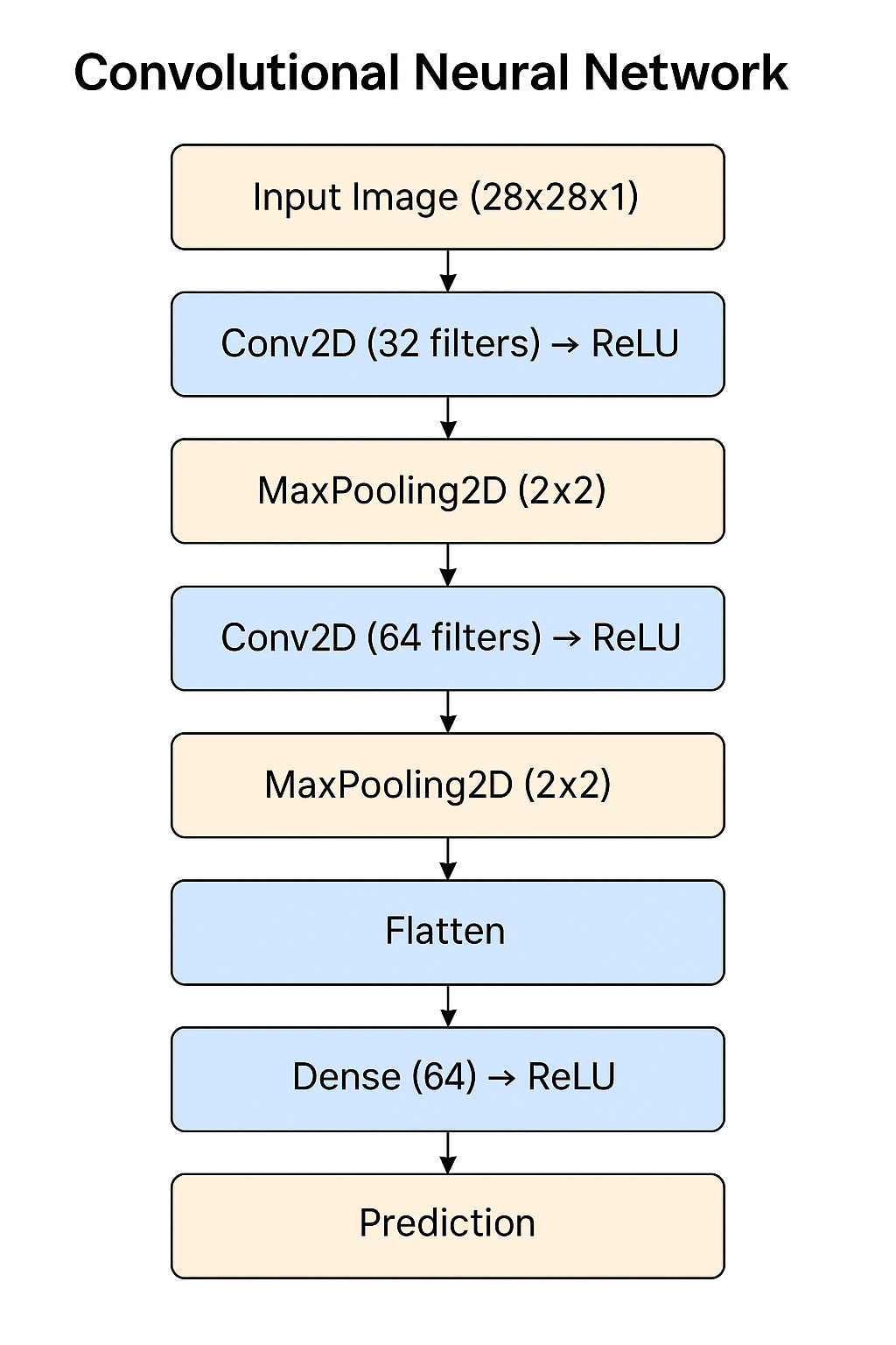
Step 1: Input Image

• Provide the input image of size (28 x 28 x 1).

Step 2: Convolution Layer 1

• Apply Conv2D with 32 filters to extract features.

Step 3: Activation - ReLU

• Apply ReLU Activation Function on the output of Conv2D (32 filters).

Step 4: MaxPooling Layer 1

• Perform MaxPooling2D (2x2) to downsample the feature map from Step 3.

Step 5: Convolution Layer 2

• Apply Conv2D with 64 filters on the output from Step 4 for deeper feature extraction.

Step 6: Activation - ReLU

• Apply ReLU Activation Function on the output of Conv2D (64 filters).

Step 7: MaxPooling Layer 2

• Perform MaxPooling2D (2x2) on the output from Step 6 for further downsampling.

Step 8: Flatten Layer

• Flatten the output from Step 7 into a 1D vector to prepare for Dense Layers.

Step 9: Dense Layer

• Apply Dense Layer with 64 neurons for learning complex patterns.

Step 10: Activation - ReLU

• Apply ReLU Activation on the output of Dense Layer.

Step 11: Output Layer - Prediction

• Perform final prediction using Softmax to classify the input image into one of the target classes.

Explanation:

1. Import Required Libraries

import tensorflow as tf
from tensorflow.keras import layers, models
from tensorflow.keras.datasets import mnist
from tensorflow.keras.utils import to_categorical

Purpose:

• tensorflow: Deep Learning Library

• layers: For CNN layers like Conv2D, MaxPooling2D, etc.

• models: To create a Sequential model

• mnist: Dataset of handwritten digits (0 to 9)

• to_categorical: Converts labels like 5 → [0 0 0 0 0 1 0 0 0 0] (One Hot Encoding)

2. Load MNIST Dataset

(X_train, y_train), (X_test, y_test) = mnist.load_data()

• X_train → 60,000 training images of size 28x28 pixels

• y_train → 60,000 labels (digits 0 to 9)

• X_test → 10,000 test images

• y_test → 10,000 test labels

3. Data Preprocessing

X_train = X_train.reshape((X_train.shape[0], 28, 28, 1)) / 255.0
X_test = X_test.reshape((X_test.shape[0], 28, 28, 1)) / 255.0

Why reshape?

CNN expects input as:

(batch_size, height, width, channels)

Here:

• 28x28 image with 1 channel (Grayscale)

Why divide by 255?

To normalize pixel values between 0 and 1 (since original pixel values are 0-255).

4. Convert Labels to One-Hot Encoding

y_train = to_categorical(y_train)
y_test = to_categorical(y_test)

For example:

• Label 5 becomes: [0 0 0 0 0 1 0 0 0 0]

5. Build the CNN Model

model = models.Sequential([
    #Layer 1: Convolution Layer
    layers.Conv2D(32, (3, 3), activation='relu', input_shape=(28, 28, 1)),
    
    layers.MaxPooling2D((2, 2)),
    layers.Conv2D(64, (3, 3), activation='relu'),
    layers.MaxPooling2D((2, 2)),
    layers.Flatten(),
    layers.Dense(64, activation='relu'),
    layers.Dense(10, activation='softmax')
])

What is models.Sequential([])?

A Sequential model is a linear stack of layers — you build the model layer-by-layer in order.

Layer 1: Convolution Layer

layers.Conv2D(32, (3, 3), activation='relu', input_shape=(28, 28, 1))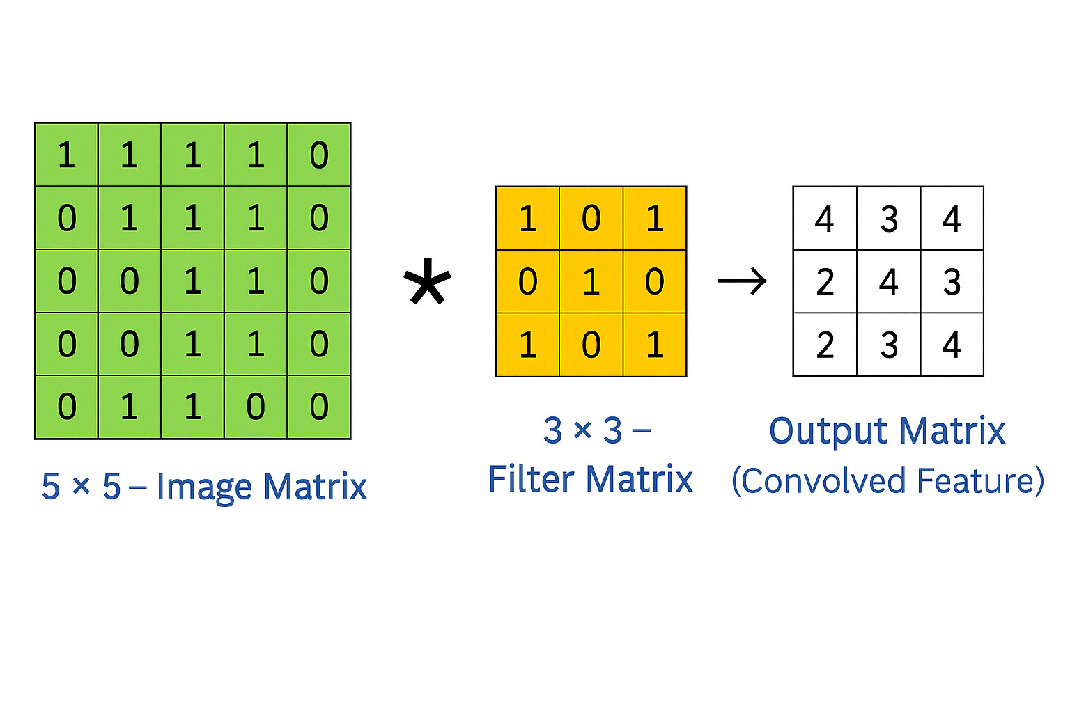

Meaning:

• 32 filters (also called kernels)

• Each filter is of size 3x3

• ReLU activation is applied after convolution

• Input shape is 28x28x1 (1 channel → grayscale image)

Parameters:

• filters: Number of filters (32 features will be learned)

• kernel_size: Size of each filter (3x3 window moves over the image)

• activation: Applies a non-linear function (ReLU = max(0, x))

• input_shape: Shape of input data

Analogy:

• Think of filters as magnifying glasses that scan an image for features.

  • One filter might detect vertical edges

  • Another may detect horizontal edges

  • It's like scanning an X-ray through different lenses to detect bones, tissues, etc.

What is a Filter?

A filter (or kernel) is a small matrix (e.g., 3x3) that slides over the image and performs a mathematical operation (convolution) at every step.

Each filter extracts a different feature from the image — such as:

• Edges

• Curves

• Texture

• Patterns (like corners)

Example: One 3x3 Filter

Let's say you have a 3x3 filter:

[[-1, -1, -1], [ 0, 0, 0], [ 1, 1, 1]]

This is a Sobel filter, and it's used to detect horizontal edges.

If you slide this filter over an image, you'll get a feature map that highlights horizontal patterns in the image.

Now Imagine: 32 Filters

Each filter is randomly initialized and learns a specific pattern during training.

So:

• Filter 1 may detect vertical lines

• Filter 2 may detect diagonal edges

• Filter 3 may detect circles or loops (like in digit 8)

• ...

• Filter 32 may detect texture, corner orientation, or stroke width

Output Shape

If the input image is 28x28x1, the output after:

Conv2D(32, (3, 3), activation='relu')

Will be: 26x26x32

Why 26?
Because a 3x3 filter reduces the image dimension:

New size = (Old size - Filter size) + 1 = (28 - 3) + 1 = 26

Why 32?
Because we applied 32 filters → We get 32 such feature maps.

Visual Example (Text-based)

Original (3x3 part of image):

[200, 200, 200] [ 0, 0, 0] [200, 200, 200]

Apply Horizontal Edge Filter:

[-1, -1, -1] [ 0, 0, 0] [ 1, 1, 1]

Output of convolution:

= (200*-1 + 200*-1 + 200*-1) + (0*0 + 0*0 + 0*0) + (200*1 + 200*1 + 200*1) = -600 + 0 + 600 = 0

That one output becomes a pixel in the feature map.

---

Layer 2: Max Pooling

layers.MaxPooling2D((2, 2))

This layer reduces the spatial size (width and height) of the feature maps from the convolutional layers — by selecting only the most important values from a patch of values.

Meaning:

• Reduces the size of the feature map.

• From 26x26 → 13x13 (if stride=2)

Parameters:

• pool_size=(2, 2): Looks at each 2x2 patch and picks the maximum value

Analogy:

• Like zooming out on a photo — you keep the most important pixels (e.g., the sharpest edges) and discard the rest.

• Imagine compressing a photo for faster loading while still keeping important visual information.

Purpose of Max Pooling

• Downsample the feature maps

• Reduce computation

• Prevent overfitting

• Keep important features

• Retain translation invariance (important feature doesn't move much if the image shifts slightly)

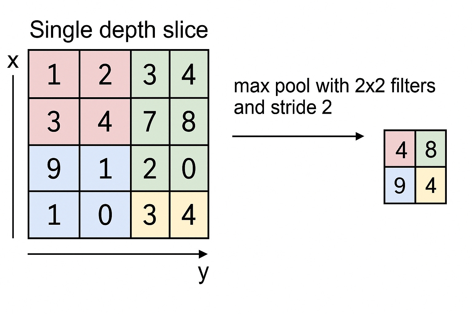
Example with a Simple 4x4 Feature Map

Suppose you have a 4x4 output from a Conv2D layer:

[ [1, 3, 2, 4],
  [5, 6, 7, 8],
  [2, 1, 4, 3],
  [0, 2, 5, 6] ]

Now apply:

MaxPooling2D(pool_size=(2, 2))

It divides the matrix into 2x2 non-overlapping patches:

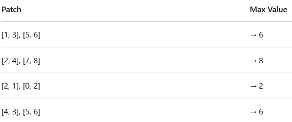
So the output becomes:

[ [6, 8],
  [2, 6] ]

Result: Original 4x4 becomes 2x2 — dimensions halved.

Parameters of MaxPooling2D((2, 2))

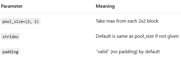
Behind the Scenes: How It Works

1. Slides a 2x2 window across the input feature map

2. For each 2x2 patch, finds the maximum value

3. Places that max value in the new pooled feature map

This process:

• Shrinks the image/feature map

• Keeps only strongest features

---

Layer 3: Another Convolution

layers.Conv2D(64, (3, 3), activation='relu')

• This time we’re using 64 filters

• No need to specify input_shape again — it's inferred from the previous layer.

Analogy:

• Deeper filters now learn more complex patterns: not just edges but maybe shapes like eyes, noses, digits, etc.

• It’s like a detective going from “I see lines” → “I see a face!”

Why 64 Filters?

• In early layers (like Conv2D(32, ...)) → filters learn basic features like edges and corners.

• As we go deeper (like Conv2D(64, ...)) → filters learn more detailed and abstract features like:

  • Loops in digit '8'

  • Tails in '9'

  • Closed circles in '6' and '0'

So, 64 filters → allow the model to learn 64 different patterns or features from the earlier 32-feature representation.

Example Walkthrough

Let’s assume the output from the last layer is of shape:

13 x 13 x 32

(From previous MaxPooling layer)

Now we apply:

Conv2D(64, (3, 3))

Step-by-Step:

• Each 3x3 filter slides across each of the 32 input channels

• 64 different filters will generate 64 new feature maps

• The output shape becomes:

(13 - 3 + 1) x (13 - 3 + 1) x 64 = 11 x 11 x 64

So now we have: ✔ Smaller spatial dimensions
✔ More depth (channels) — now 64

ReLU Activation

ReLU stands for:

Rectified Linear Unit → f(x) = max(0, x)

• ReLU replaces negative values with 0

• Keeps positive values as is

Visualization Idea (Text-based)

Imagine this small 3x3 patch of previous output:

[ [0, 1, 2], [2, 1, 0], [1, 3, 1] ]

And a random 3x3 filter:

[ [1, 0, -1], [1, 0, -1], [1, 0, -1] ]

Do element-wise multiplication and sum:

= 0*1 + 1*0 + 2*(-1) + 2*1 + 1*0 + 0*(-1) + 1*1 + 3*0 + 1*(-1) = 0 + 0 -2 + 2 + 0 + 0 + 1 + 0 -1 = 0

Then apply ReLU:

ReLU(0) = 0

---

Layer 4: Max Pooling Again

layers.MaxPooling2D((2, 2))

• Again, reducing the size by half.

• Helps keep only essential features and reduces computation.

---

Layer 5: Flatten

layers.Flatten()

What it does:

• Converts 2D feature maps to 1D array to feed into dense layers.

Example:

• If input was 5x5x64 → output becomes 1600 neurons in 1D

Analogy:

• Imagine converting a chessboard into a row of 64 squares. You're unrolling a mat to feed it to a classifier.

1. Purpose of Flatten Layer in CNN:

Flatten Layer → Converts multi-dimensional data (output from Conv2D and Pooling layers) into a one-dimensional vector (1D array).

It acts like a "Bridge" between the Convolutional Layers (Feature Extraction) and the Dense Layers (Classification).

2. What Problem does Flatten Solve?

CNN Feature Map Output looks like this:

Example:

Shape = 5 x 5 x 64

• 5 Rows

• 5 Columns

• 64 Filters (Depth)

This is like a 3D cube of numbers.

But —
Dense (Fully Connected) Layers can only take:

1D Array (Vector) like [x1, x2, x3, ..., xn]

Flatten layer does this conversion.

Real Example:

Input Feature Map from previous layer:

5 x 5 x 64 = 1600 numbers

Flatten Layer will convert:

[ [ [x1, x2, ..., x64],
    ...
    ...
  ],
  [ [x65, x66, ..., x128],
    ...
  ],
  ...
]

→ into:

[x1, x2, x3, ..., x1600]

Now this 1D vector can go into:

layers.Dense(64, activation='relu')

Output Size after Flatten:

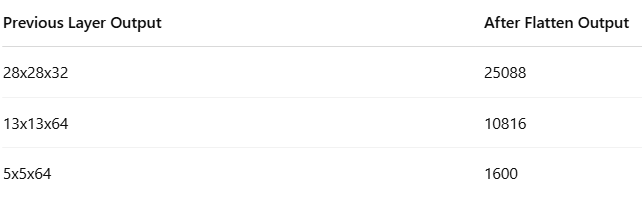
Formula:

Output = rows x columns x depth

---

Layer 6: Dense Layer (Fully Connected)

layers.Dense(64, activation='relu')

What is it?

• A fully connected layer with 64 neurons.

• Each of the 1600 outputs from the Flatten() layer connects to all 64 neurons.

• Applies ReLU activation.

Purpose:

• Combines and learns relationships between all extracted features.

• Helps detect patterns like:

  • “If this edge exists AND this curve exists, then it's probably a 9”

Analogy:

• Like a team of 64 detectives analyzing 1600 clues and deciding which are important.

Output Shape:

• Input: 1600 values (from Flatten)

• Output: 64 values

---

Layer 7: Output Layer

layers.Dense(10, activation='softmax')

What is it?

• Another fully connected layer, this time with 10 neurons — one for each class (digit 0 to 9).

• Applies Softmax activation.

What Softmax Does:

It converts raw values into probabilities that sum up to 1.

Example input to softmax:

[3.2, 1.1, -2.0, 0.9, 5.0, 2.5, 1.2, 3.1, 0.7, 0.5]

Softmax Output:

[0.01, 0.00, 0.00, 0.01, 0.92, 0.03, 0.01, 0.01, 0.00, 0.01]

→ So, this means the model is 92% confident it's class 4.

Final Prediction Output

Example:

Prediction = [0.01, 0.00, ..., 0.92, 0.03]

Means:

• Class 0: 1% chance

• Class 1: 0%

• ...

• Class 4: 92%

• Class 9: 3%

✅ So the model predicts:

Predicted Digit = np.argmax(Prediction) # Output: 4

---

6. Compile the Model

model.compile(optimizer='adam', loss='categorical_crossentropy', metrics=['accuracy'])

• Optimizer: adam → Adaptive Learning Rate Optimizer

• Loss: categorical_crossentropy → For Multi-Class Classification

• Metrics: accuracy

---

7. Train the Model

model.fit(X_train, y_train, epochs=5, batch_size=64, validation_split=0.1)

• Trains the model for 5 iterations (Epochs)

• Batch size of 64

• 10% of training data used for validation.

---

8. Evaluate the Model

test_loss, test_acc = model.evaluate(X_test, y_test) print(f"Test Accuracy: {test_acc:.2f}")

Evaluates the model performance on unseen test data.

Final Output:

Epoch 1/5 Train Accuracy increasing... Test Accuracy: 0.98

---

Next Steps:

Ready to master CNNs?
Don't stop here—explore, experiment, and build your own convolutional neural networks. Check out my other deep learning tutorials and practical guides on AI, Python, and Machine Learning.

Have questions or want to share your CNN journey?
Drop your insights and experiences in the comments or connect with me on LinkedIn—I’d love to hear from you!

Keep exploring, keep innovating! 🌟
Happy Learning!

---

For more in-depth technical insights and articles, feel free to explore:

Girish Central

• LinkTree: GirishHub – A single hub for all my content, resources, and online presence.

• LinkedIn: Girish LinkedIn – Connect with me for professional insights, updates, and networking.

Ebasiq

• Substack: ebasiq by Girish – In-depth articles on AI, Python, and technology trends.

• Technical Blog: Ebasiq Blog – Dive into technical guides and coding tutorials.

• GitHub Code Repository: Girish GitHub Repos – Access practical Python, AI/ML, Full Stack and coding examples.

• YouTube Channel: Ebasiq YouTube Channel – Watch tutorials and tech videos to enhance your skills.

• Instagram: Ebasiq Instagram – Follow for quick tips, updates, and engaging tech content.

GirishBlogBox

• Substack: Girish BlogBlox – Thought-provoking articles and personal reflections.

• Personal Blog: Girish - BlogBox – A mix of personal stories, experiences, and insights.

Ganitham Guru

• Substack: Ganitham Guru – Explore the beauty of Vedic mathematics, Ancient Mathematics, Modern Mathematics and beyond.

• Mathematics Blog: Ganitham Guru – Simplified mathematics concepts and tips for learners.